Introduction to Machine Learning

Machine learning, a branch of artificial intelligence, concerns the construction and study of systems that can learn from data. With a deluge of machine learning sources both online and offline, a newcomer in this field would simply get stranded due to indecisiveneww. This post is for all Machine Learning Enthusiasts who are not able to find a way to understand Machine Learning (ML).

This tutorial doesn’t require you to have a good deal of understanding of optimizations, linear algebra or probability. It is about learning basic concepts of Machine Learning and coding it. I would be using a python library scikit-learn for various ML applications.

Let’s start with a very simple Machine Learning algorithm Linear Regression.

Linear Regression

Linear Regression is an approach to the model the relationship between a scalar dependent variable y and one or more indenpendent variable X.

$\begin{align} y = \left [ \begin{array}{c} y^1 \\ \vdots \\ y^n \end{array}\right] \hspace{10 mm} X = \left[ \begin{array}{cc} X^1_1 \dots X^1_m \\ \vdots \ddots \vdots \\ X^n_1 \dots X^n_m \end{array} \right] \end{align}$

n = number of samples
m = number of features

A linear regression model assumes that the relationship between the dependent variable $y_i$ and independent variable $X_i$.

$\begin{align} y^i = a_0 + a_1*X^i_1 + a_2*X^i_2 + \dots + a_m*X^i_m \end{align}$ $\begin{align} y = \left[ \begin{array}{cc}1 \hspace{3 mm} X^1_1 \hspace{3 mm} \dots \hspace{3 mm} X^1_m \\ 1 \hspace{3 mm} X^2_1 \hspace{3 mm} \dots \hspace{3 mm} X^2_m \\ \vdots \hspace{3 mm} \ddots \hspace{3 mm} \vdots \\ 1 \hspace{3 mm} X^n_1 \hspace{3 mm} \dots \hspace{3 mm} X^n_m \end{array} \right] \left[ \begin{array}{c} a_0\\ a_1\\ \vdots \\ a_m \end{array} \right]^T \end{align}$

a₀, a₁, …. , a_m are some constants.

Linear Regression with One Variable (Univariate)

First we start with modelling a hypothesis $h_\theta(X)$.

$\begin{align} h_\theta(X) = \theta_0 + \theta_1*X \end{align}$

The objective of linear regression is to correctly estimate the values of $\theta_0$ and $\theta_1$ such that $h_\theta(X)$ approximates to $y$ . But how to do that?. For this we define a cost function or error function $J(\theta)$ as:

$\begin{align} J(\theta) = \frac{1}{2n}\sum_{i=1}^n (h_\theta(X^i) - y^i) \end{align}$

Linear Regression models are often fitted using least squares approach i.e. by minimizing squared error function (or by minimizing a penalized version of the squares error function). For minimizing the error function we use the Gradient Descent Algorithm. This method is based on the observation that if a function $f(x)$ is defined and differentiable in the neighborhood of a point $\beta$ , then $f(x)$ decreases fastest if one goes from $\beta$ in the direction of negative gradient of $f(x)$ at $\beta$ . So, we can find the minima by updating the value of $\beta$ as:

$\begin{align} \beta := \beta - \alpha\nabla f(\beta) \end{align}$

Where $\alpha$ is the step size.
Using the above concept, we can find the values of $\theta_0$ and $\theta_1$ as:

$\begin{align} \theta_0 := \theta_0 - \alpha\frac{\partial J(\theta)}{\partial \theta_0}\\ \theta_1 := \theta_1 - \alpha\frac{\partial J(\theta)}{\partial \theta_1} \end{align}$

Here $\alpha$ is called as the learning rate.
Replacing the values of $\frac{\partial J(\theta)}{\partial \theta_i}$ as

$\begin{align} \frac{\partial J(\theta)}{\partial \theta_i} = \frac{1}{n}\sum_{j=1}^n(h_\theta(X^j) - y^j)X_i^j \end{align}$

We can have a general formula for finding optimal value for any $\theta_i$ as:

$\begin{align} \theta_i := \theta_i - \alpha\frac{1}{n}\sum_{j=1}^n(h_\theta(X^j) - y^j)X_i^j \end{align}$

Phew!!!. A lot of mathematics, right?. But where is the code?.

Let’s get our hands on some coding. For this tutorial I would be going to use scikit-learn for machine learning and matplotlib for plotting.

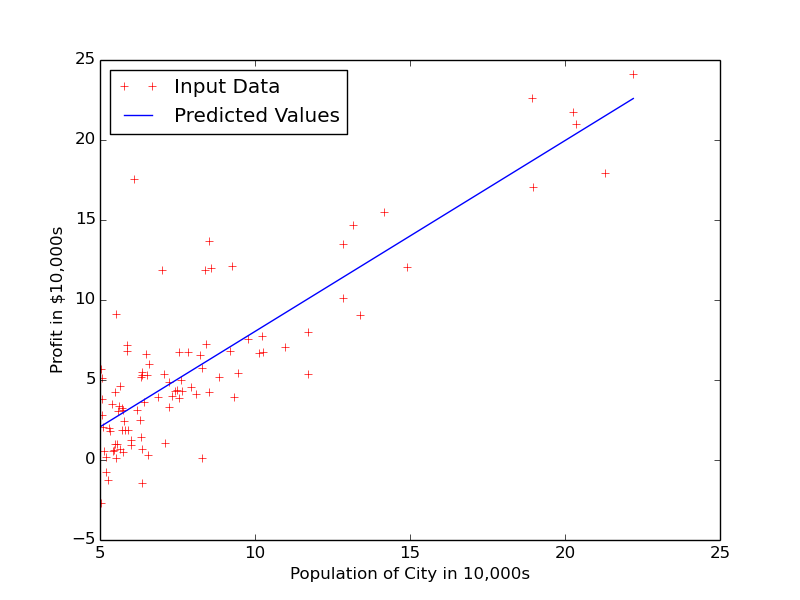
Suppose, for a hypothetical city FooCity, population in 10,000s and profit in $10,000 are available. We want to predict price of a house of particular size.

load_data

import numpy as np
import matplotlib.pyplot as plt

input_file = open('example1.txt')
lines = input_file.readlines()

X = [map(float, line.strip().split(','))[0] for line in lines]
#X : size of house
X = np.array(X)
#converting X from a list to array
X = X.reshape(X.shape[0], 1)
#reshaping the X from size(97, ) to (97, 1)

y = [map(float, line.strip().split(','))[1] for line in lines]
#y : price of house
y = np.array(y)
#converting y from a list to array
y = y.reshape(y.shape[0], 1)
#reshaping the y from size(97, ) to (97, 1)

plt.plot(X, y, 'r+', label='Input Data')
#plotting house size vs house price
plt.ylabel('Profit in $10,000s')
plt.xlabel('Population of City in 10,000s')
plt.show()

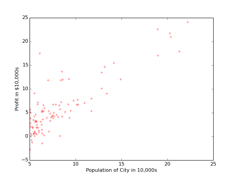
It is visible from the plot that Population and Profit are varying linearly, so we can apply linear regression and predict profit for a given population.
For performing Linear Regression we have to use LinearRegression class available in sklearn.linear_model.

linear_regression

from sklearn.linear_model import LinearRegression

clf = LinearRegression()
clf.fit(X, y)
#linear regression using scikit-learn is very simple.
#just call the fit method with X, y

We can now predict the value of Profit for any Population(such as 15.12*10000) as clf.predict(15.12).

plot

x_ = np.linspace(np.min(X), np.max(X), 100).reshape(100, 1)
#x : array with 100 equally spaced elements starting with 
#min value of X upto max value of X
y_ = clf.predict(x_)
plt.plot(x_, y_, 'b', label='Predicted values')
plt.legend(loc='best')

Next, we would be going for Multivariate Linear Regression.

Pythonic Musings

Data Analysis and Machine Learning in Python

Introduction to Machine Learning

Linear Regression

Linear Regression with One Variable (Univariate)

Comments